Effective Ways to Sum a Column in Excel for Accurate Data Analysis in 2025

Understanding the Sum Function in Excel

When it comes to data analysis in Excel, mastering the **sum function** is essential. The simplicity of summing values allows users to quickly calculate the total of a column, making it one of the most utilized features within Microsoft Excel. It’s crucial to know how to sum numbers effectively to ensure your calculations are accurate and reliable. Here, we delve into various methods to sum columns in Excel while enhancing your data management skills.

Basic Sum Formula: The Starting Point

The most fundamental way to sum a column in Excel is by using the **excel sum formula**. This is a straightforward approach where you can use the syntax =SUM(range). For instance, if you want to calculate the total of values from cell A1 to A10, you would enter =SUM(A1:A10) in another cell. This will provide an aggregate of all numbers in the specified range. Mastering this basic formula sets a solid foundation for performing more complex calculations, enhancing your efficiency in **excel calculations** and data analysis.

Using AutoSum for Quick Calculations

For those who prefer a more convenient method, Excel provides the **excel auto sum** feature, which can substantially expedite the summing process. By selecting a cell directly below or to the right of the data range to be summed, and then clicking the AutoSum button in the toolbar (often represented by the Σ symbol), Excel will automatically suggest a sum range. This feature not only simplifies the process but also reduces errors that may occur while manually selecting ranges. Utilizing this tool can help improve productivity when working with spreadsheets and pre-defined data formats.

Dynamic Sum Ranges: Adapting to Changing Data Sets

In many instances, datasets may change, and the ability to create a **dynamic sum in Excel** becomes vital. This can be achieved by using Excel tables, which automatically adjust the referenced ranges as new data is added or removed. To do this, convert your data range to an Excel table by selecting it and navigating to the “Insert” tab, then clicking “Table.” Once established, use the table name in your sum formula, such as =SUM(TableName[ColumnName]), ensuring that your calculations always reflect the latest data inputs. Keeping up with these modern techniques not only streamlines your accounting processes but also fortifies your skills in managing accounts efficiently.

Advanced Summing Techniques in Excel

Once you’re comfortable using the basic functions, there are advanced summing techniques to uncover more powerful insights from your data. This section will explore conditions under which you might need more than just a basic sum, showcasing features such as the **sumif excel** and **sumifs function**, both critical for flexibility in data evaluation.

Conditional Summing with SUMIF

The **SUMIF** function allows users to sum values based on specified criteria. For example, if you want to sum values in a column only if corresponding cells meet a certain condition, you would use the syntax =SUMIF(range, criteria, sum_range). A practical example would be summing sales amounts that exceed $500 by inputting =SUMIF(B2:B10, ">500", C2:C10), where B2:B10 contains the sales figures and C2:C10 contains the amounts you want to sum. This powerful tool assists in targeting specific data subsets, crucial for **excel data reporting** and insightful decision-making.

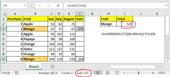
Leveraging SUMIFS for Multiple Criteria

For scenarios involving multiple conditions, the **SUMIFS** function is invaluable. Similar to SUMIF, it enables summation based on several criteria, following the format =SUMIFS(sum_range, criteria_range1, criteria1, [criteria_range2, criteria2], …). If you’re tracking data such as total sales made by a certain representative within a specific timeframe, this function becomes essential. Say you want to total the sales from January for a particular salesperson; your formula might look something like this: =SUMIFS(C2:C10, A2:A10, "January", B2:B10, "John Doe"). Implementing such sophisticated functions allows for comprehensive analysis and refined strategies in **data visualization in Excel**.

Utilizing Array Functions for Complex Calculations

For users seeking advanced calculations, considering excel array functions can be a game-changer. These allow you to perform multiple operations on one or more items in an array, drastically enhancing your ability to conduct intricate data evaluations. An example would include using an array formula to sum products conditionally. By entering =SUM((A2:A10>50)*(B2:B10)) as an array entry, pressing Ctrl+Shift+Enter will perform the summation only where the values in range A2:A10 exceed 50. Grasping the implications and execution of these functions can significantly upgrade how you view and relate **improving excel skills** to data interpretation and management.

Visualizing Results from Summation in Excel

Once you’ve effectively calculated sums, it’s important to visualize this data in a way that enhances interpretation. Excel offers various functionalities that allow users to transform numerical aggregates into visual representations, such as charts and graphs, which foster clearer communication of data trends.

Creating Pivot Tables for Dynamic Insights

Using **excel pivot tables** is one of the most powerful methods to analyze your summed results dynamically. Pivot tables allow you to summarize large datasets interactively, displaying the sums based on various parameters. By dragging fields into the Rows and Values areas, you can affordably rearrange your data and modify the sums that populate based on your specifications. This flexibility serves as a massive advantage in **excel financial analysis**, letting you identify patterns that inform better decision-making.

Excel Charts and Graphs for Summation Data

Creating charts helps visualize sums for presentations or reports. After summing your data, go to the “Insert” tab, select your desired chart type, and let Excel convert your summed values into an easy-to-digest format. This visual approach provides stakeholders with an immediate grasp of trends and totals, essential in executive summaries and **business intelligence with Excel** applications.

Tips for Effective Data Summarization

• Always double-check your ranges and criteria to prevent errors in your output.
• Understand the implications of using Excel tables and consider leveraging them for dynamic sum ranges.
• Familiarize yourself with visual tools in Excel, as they complement successful Data Analysis.
• Take advantage of Excel’s built-in tutorials and online resources to further enhance your skills and techniques.

Key Takeaways

Summing columns in Excel is a fundamental skill that enhances data analysis efficiency. Mastering the basics, using AutoSum, and exploring functions like SUMIF and SUMIFS, positions you well in financial management. Moreover, integrating visual tools like pivot tables and charts elevates reporting capabilities, ensuring clarity and accessibility of your data insights.

FAQ

1. What is the fastest method to sum a column in Excel?

The fastest method is to use the **Excel AutoSum** feature. Simply place your cursor in the cell below the column of numbers you wish to sum and click the AutoSum button. Excel will suggest a range to sum, making it a quick and efficient option for totaling data quickly.

2. Can I sum numbers based on specific criteria in Excel?

Yes! The **SUMIF** function allows you to sum numbers based on specific criteria. For instance, you can sum all sales that exceed a certain threshold by utilizing =SUMIF(sales_range, criteria, sum_range). This provides flexibility for precise calculations needed in data-driven evaluation.

3. How do I create a dynamic sum range in Excel?

To create a dynamic sum range, consider converting your dataset into an Excel table. Then, you can use the table name in your sum formulas, such as =SUM(TableName[ColumnName]). This will automatically adjust the range as you add or remove data within the columns of the table.

4. What is the difference between SUMIF and SUMIFS?

**SUMIF** is used to sum a range based on a single criterion, whereas **SUMIFS** allows you to sum a range based on multiple criteria. This differentiates them in capabilities, making SUMIFS better suited for complex summation needs across various parameters.

5. How can I visualize my summed data in Excel?

You can visualize summed data by using charts and graphs. After calculating your total sums, select your desired chart type from the “Insert” tab. This visualization effectively communicates trends and insights stemming from your summed values, essential for conveying information to stakeholders.